High Reynolds Number in Lid Driven Cavity

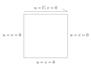
The lid-driven cavity problem has long been used a test or validation case for new codes or new solution methods. The problem geometry is simple and two-dimensional, and the boundary conditions are also simple. The standard case is fluid contained in a square domain with Dirichlet boundary conditions on all sides, with three stationary sides and one moving side (with velocity tangent to the side).

Difficulty rises when Reynolds Number becomes large. If we write N-S Equation into non-dimensional form, it becomes:

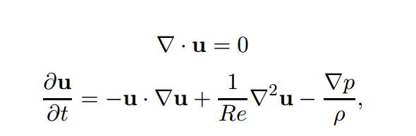
Here, the inverse of Reynolds number represent non-dimensional viscosity. Larger the Reynolds Number, slower the information propagates. Therefore, for the solution to reach steady state, a later instant should be simulated for larger Reynolds Number. If the time marching step is constant, then a lot more time steps are needed, resulting in more running time.

This difficulty could be overcome by adjusting the time step with respect to Reynolds Number. It is obvious that both convective term and diffusion term exist in the equation, which means that two CFL conditions are imposed on time marching step:

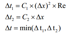
The first CFL condition (dominant for large RE cases) become less restrictive as Re grows. This enables us to use large time step for larger Reynolds Number, making it less time-consuming.

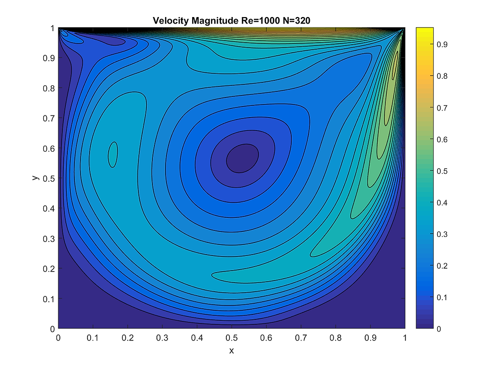
If we refer to similarity solution in Stokes’ first problem, we can estimate the time domain we need to calculate: 0 < t < Constant * Reynolds Number. Admittedly, this is not exactly correct due to the lack of similarity solution in this problem caused by boundary condition (Please refer to Stokes’ First Problem for further information), but it is still a good estimation that could be verified by numerical experiment. If we follow the ideas above to choose time domain and time step, time required to complete the simulation for different Reynolds Number is almost the same. The result for Re=1000 has been shown: